A straightforward approach to estimating task duration is the PERT (Program Evaluation Review Technique) weighted average method. This technique calculates task duration using a weighted average estimate, allowing for the consideration of various types of estimates—such as probabilistic values, ranges, and areas with limited definition.
The method is based on the Beta distribution model, which is well-suited for modeling events constrained within a defined interval of minimum and maximum values. Because of its ability to describe task completion times within specific bounds, the Beta distribution is widely used in PERT, CPM, and other project planning and control systems.
The term weighted average means that the equation uses weighted factors to calculate the expected task duration.
The equation and process modelling a task for PERT is the following:
E=(O+4M+P)/6 (equation)
E= Expected Value
O= Optimistic Value (this is equivalent to a minimum value)
M= Most Likely Value
P= Pessimistic Value (this is equivalent to a maximum value)
(i) Fist, acquire estimates for the pessimistic value, most likely value and optimistic value time to completion. For example, let's suppose that: P=20 programmer days M=12.5 programmer days O=10 programmer days
(ii) Then, using the "PERT Weighted Average" equation: E=[(10+4(12.5)+20]/6 = 13.333 programmer days = expected task duration = mean value.
PERT Distribution background
The PERT distribution is a probabilistic model, based on Beta
Distribution, and it derives its estimates based on the probability of
occurrence (i.e., chance or possibility - if an event is likely to happen, we
say it is probable. On the other hand, if it is not likely to happen, we say it
is improbable. Directly or indirectly, probability of occurrence plays a role
in the all activities. Probability of occurrence of any event will be a number
between 0 and 1. Events that are unlikely will have a probability near 0, and
events that are likely to happen have probabilities near 1).
The Beta Model is a flexible yet continuous distribution, defined on
the interval (0, 1), that places value on the event itself and the interval
between events. Because it accounts for a degree of randomness, it is highly
useful in determining likely event durations (time estimates for tasks). In other words, PERT can derive a task
duration with a high probability of accuracy based on three values provided by
experts estimates (pessimistic, optimistic and most likely). But, it’s still an
estimate because it is only as good as the estimates used in the computation.
Probability Density Function Graphical Profiles
The Beta Distribution is parameterized by two positive shape
parameters, denoted by alpha and beta. It can take on different shapes depending on
the values of the two parameters. The domain of the beta distribution can be
viewed as a probability to describe the distribution of an unknown probability value. The range depends on the chosen shape
parameters.
Typically, the general form of a distribution model is given in
terms of location and scale parameters. The Beta function is different in that the general
distribution model is defined in terms of the lower and upper bounds. However,
the location and scale parameters can be defined in terms of the lower and
upper limits as follows:
location = a
|
scale = b – a
|
Location and scale parameters
These parameters, location and scale, are used in modeling
applications.
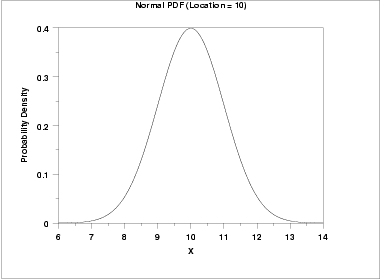
The effect of the location parameter is to translate the graph,
relative to the standard normal distribution, 10 units to the right on the
horizontal axis. A location parameter of -10 would have shifted the graph 10
units to the left on the horizontal axis. That is, a location parameter simply
shifts the graph left or right on the horizontal axis.
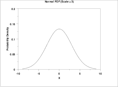
The effect of a scale parameter greater than one is to stretch the Probability
Density Function. The greater the magnitude, the greater the stretching. The
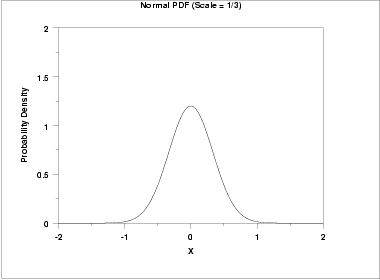
effect of a scale parameter less than one is to compress the function.
The compressing approaches a spike as the scale parameter goes to
zero. A scale parameter of 1 leaves the function unchanged (if the scale
parameter is 1 to begin with) and non-positive scale parameters are not
allowed.
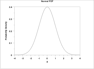
The standard form of any distribution is the form that has location
parameter zero and scale parameter one.
Ex.1: the following graph has a location of 0 and scale of 1.
Ex.2: the following graph has a location
of 10 and scale of 1.
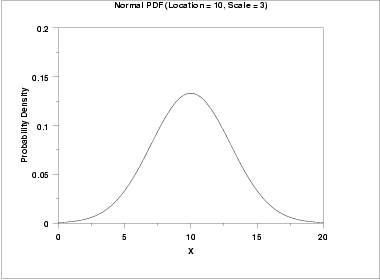
Ex.3: the next plot has a scale
parameter of 3 (and a location parameter of zero). The effect of the scale
parameter is to stretch out the graph. The maximum y value is approximately
0.13 as opposed 0.4 in
the previous graphs. The y value, i.e., the vertical axis value, approaches
zero at about (+/-) 9 as opposed to (+/-) 3 with the first graph.
Ex.4: In contrast, the next graph has a
scale parameter of 1/3 (=0.333). The effect of this scale parameter is to
squeeze the function. That is, the maximum y value is approximately 1.2 as
opposed to 0.4 and the y value is near zero at (+/-) 1 as opposed to (+/-) 3.

Ex.5: The following graph shows the
effect of both a location and a scale parameter. The plot has been shifted
right 10 units and stretched by a factor of 3.
The Beta distribution in its standard form ranges from zero to one and
takes a wide range of shapes (see the Probability Density Function Graphical
Profiles graph on top). Moreover, it can an also be rescaled and shifted to
create distributions with a wide range of
shapes and over any finite range
for various applications. For example, it’s used to model expert opinion in the
form of the PERT distribution.
The PERT distribution comes out of the need to describe the
uncertainty in tasks during the development of a complex project having thousands
of tasks. Estimates were needed to be made intuitively, quick and consistent in
approach.
The Beta distribution can be rescaled to model a variable that runs
from a to b by using the following formula:
x = a + B(a ,b) * (b - a)
This is the four-parameter version of the Beta distribution. A version
of this four-parameter Beta distribution is called a PERT distribution and makes
the assumption that the mean = (minimum + 4*most likely + maximum) / 6. The
default value of 4 scales the height of the distribution. This extra equation
allows the four parameters to be determined from three input values: the
minimum, most likely and maximum, which makes it ideal for modeling expert
opinion of a variable's uncertainty.
Mean= (Min+Max+4*Mode)/(4+2)
|
Using the three point estimation, estimates of the mean, standard
deviation and variance can be obtained:
Expected Time (ET) = ( Optimistic + 4 x Most likely + Pessimistic )
/ 6
Expected time (ET) = ( Min + 4 x Most likely + Max) / 6
Standard Deviation (SD) = (Max-Min)/6
Variance (V) = =SD**2 (Standard Deviation squared)
Table Example
List of all tasks lying on the critical path of a project
|
||||||
Tasks
|
Min
|
MLT
|
Max
|
ET
|
SD
|
V
|
Task A
|
||||||
Task B
|
||||||
Task C
|
||||||
(All time durations are
estimates).
Legend
-Min = Optimistic time is generally the shortest time in which the
activity can be
completed.
-Most Likely Time (MLT) is the completion time having the highest
probability.
-Max = Pessimistic time is the longest time that an activity might
require.
-SD (Standard Deviation) is the average deviation form the estimated
time (as a general rule, the higher the SD is the greater amount of uncertainty
exists).
-V (Variance) reflects the spread of a value over a normal
distribution (the SD and V will be useful in determining the probability of the
project meeting a desired completion date).
ET = Expected Time.
(Ref. NIST/SEMATECH e-Handbook of Statistical Methods)


